Array Formulas

I am doing some studying at the moment, with a view to doing my MOS 2010 exams at some stage in the future, and today I have been reading about Array Formulas. I have encountered them before but never really seen the point of them.

Simple Example

As a simple example, consider an order form:

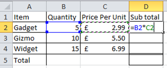
This shows the traditional way of calculating the total for each item. This formula can then be copied down each row and the total worked out by using the Sum function in row 5.

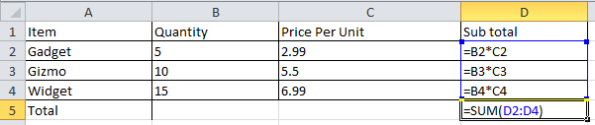
This screen shot shows the formulas, rather than their calculated values.

To create the same result using an array formula we would do the following:

1. Select cells D2:D4
2. In the formula bar, enter the formula “=B2:B4*C2:C4” (without the quotes)
3. Then press Ctrl+Shift+Enter

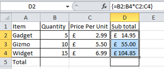
Note that pressing the key combination of Ctrl+Shift+Enter is what converts an ordinary formula to an Array Formula.

The whole thing could be simplified further by surrounding the multiplication with a SUM function.

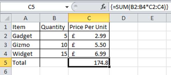
Here, the formula multiplies the values in column B by the values in column C and then sums the results.

This is all well and good but perhaps overkill when the same could be achieved using ordinary functions.

Better example

During various pieces of data analysis I have done over the years there have been occasions where most of the data has been arranged in columns but for some analysis or presentation I need to show the data in rows.

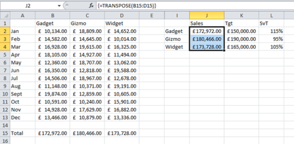
For example if I have a table of monthly sales figures like this:

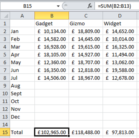
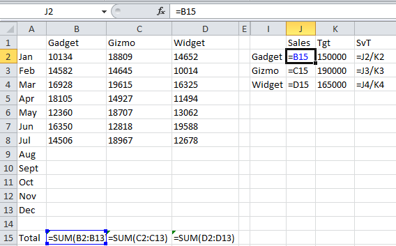
I may want to display the total sales in rows, like this:

Copy cell values

Now with only three values it would be easy enough to enter three formulas in J2:J4 such that:

Use a TRANSPOSE Array function

However, if the number of products were larger then this use of the copy cell formula would be a pain. In that case it might be easier to use the Transpose function in conjunction with an array.

Since we have three products, we would select the three cells where we want the results to appear and enter the formula =TRANSPOSE(B15:D15) and use Ctrl+Shift+Enter.

This will copy the values from cells B15:D15 into J2 to J4.

Having used a formula to copy total sales into column J, as the next months figures come in the Sales figures in column J will be automatically updated.